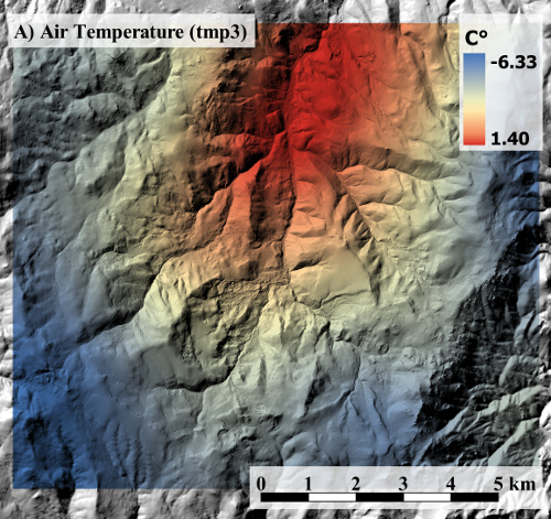
Current methods for producing spatially distributed raster grids for snow models are time consuming and often require researcher input leading to possible biased results. Empirical Bayesian kriging (EBK) is a novel approach which automates the estimation of the semi-variogram model used for kriging (Krivoruchko, 2012). Raster grids are spatially distributed rasters of various parameters which are created using point data collected at weather stations. The Image SNOwcover and mass BALance (ISNOBAL) model is used to predict seasonal snowmelt (Marks, et al., 1999, Susong et al. 1999). Using Esri's ArcGIS tools an automated approach has been developed to create raster grids for snow modeling in ISNOBAL. Kriging is a commonly used geostatistical approach for interpolating known point values to unknown points. In order to compare methods/approaches for generating raster grids, a cross validation of EBK was conducted. Results reveal an overall low mean average error (MAE) and Root Mean Square Error (RMSE) for most of the parameters. Cross validation was performed using a leave-one-out method for the 2014 water years of Johnston Draw and the 2008 water year of Reynolds Creek. The output from these automated tools can be used to force the ISNOBAL model. Simple graphical user interfaces have been developed to give researchers an easy to use tool for producing raster grids. These tools can also be used for any other model that requires a raster grid as input.
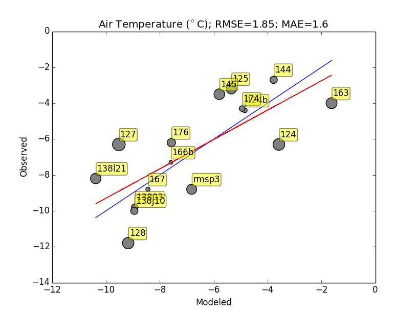
Residuals are determined using a leave-one-out method of cross validation. A python script has been written to automate the process of leave-one-out. For each time step (1-6 hour steps) several grids are interpolated leaving out one station at a time. The predicted value for the left out station is recorded as well as the observed value. The mean average error (MAE) and root mean square error (RMSE) can then be calculated using the following formulas. Graphs are produced using the python module matplotlib (Hunter, 2007). MAE is the absolute value of the difference between the modeled value and the observed value. Then calculating the mean of all values. RMSE is calculated by squaring the difference between the modeled value and the observed value. The average is calculated then square rooted. Using these two measures we can determine general model error.
The climate interpolation and cross validation toolkits used in this study can be used to produce the spatially distributed input grids required to run ISNOBAL and other spatial distributed climate models. Cross validation shows that the empirical Bayesian kriging interpolation method provides accurate results for climate parameters for the Reynolds Creek South watershed. A significant part of preparing for any virtual watershed models is the time required to prepare the climate grids to force the model. The interpolation toolkit is completely automated making it easy to produce new data to run ISNOBAL (or other distributed climate models such as PRMS (Leavesley, et al., 1983) or HydroGeoSphere (Therrien, et al., 2010)). The cross validation toolkit produces several interpolation surfaces for each time step and records the amount of time required to calculate the surface.